How is this package used? • swissrastermaps4r

Acquire raster data

In a first step, the raster maps need to be acquired and stored in a folder. Unfortunately, most of the swisstopo raster maps are behind a paywall if you aren’t part of geodata4edu. Two scales are available publicly for free (see #1):

The package is developed with a strong focus on the swisstopo raster maps and hasn’t been tested with other data. Therefore, only CRS 2056 and CRS 21781 are implemented.

Data structure

Create one folder for each maptype, scale and projection. Each folder is then named MAPTYPE_SCALE_PROJECTION (e.g. PK_25_2056). Check the function fdir_init() to get more details on the requirements for naming the folders.

Some metadata must be derived from the filename. In order to achieve this, create a text file in each folder and change the file name of that textfile to match the naming pattern on the files within the folder. For example, the 1:500’000 raster map has the filename: ‘PK500_LV95_KGRS_500_2016_1.tif’. The file structure and the corresponding “.pattern”-File should therefore look as follows:

Geodata/
├── PK_500_2056/
│   ├── PK500_LV95_KGRS_500_2016_1.tif
│   ├── AABBB_CCCC_DDDD_EEE_FFFF_G.pattern

Call get_srm4r("search_pattern_dict") to see the associated naming schema (i.e. the place-holders and their meanings). The function metainfo_from_filename is called on the file names.

Note:

The character length of the naming pattern must match the length of the filename. In this way, different naming patterns can exist within a single folder.
The naming pattern currently can’t handle variable lengths

Download package

Download and load the package. It is currently only available on github.

# install.packages("devtools")
# devtools::install_github("swissgeodata4r/swissrastermaps4r",upgrade = F)


library(swissrastermaps4r)

Scan Folder

Next, run the command fdir_init() pointing to the location (parent folder) of these maps. This command creates a “File Directory” in the package environment by scanning all folders recursively and analysing the content. All files ending with “tif” are checked for extent, number of layers and resolution. All the mentioned attributes of each raster file, along with the file path and the extent as a geometry, are stored in the variable fdir of the package environment.

fdir_init("C:/Users/rata/Geodata/01_Switzerland/01_Maps")

## Done. Scanned 632 Files (54'413.56 MB) in 12.74 (secs). -> All metadata stored in fdir (@swissrastermapEnv)

fdir_init() stored an sf object in the package’s own environment (called packageEnv). It’s a list of all raster files, stored with their extent, scale, resolution and other information (see fdir_init()).

ls(envir = swissrastermapEnv)

## [1] "fdir"                "search_pattern_dict"

Retrieve raster (example 1)

Now let’s look at an example where this package actually comes to some use. Say you want to plot a map of the largest cities in Switzerland. There is a sample dataset included in the package with name, location and size of the 10 largest cities in Switzerland.

data("sample_points")
data("switzerland")


sample_points

## Simple feature collection with 10 features and 2 fields
## geometry type:  POINT
## dimension:      XY
## bbox:           xmin: 2500063 ymin: 1099230 xmax: 2746142 ymax: 1267460
## epsg (SRID):    2056
## proj4string:    +proj=somerc +lat_0=46.95240555555556 +lon_0=7.439583333333333 +k_0=1 +x_0=2600000 +y_0=1200000 +ellps=bessel +towgs84=674.374,15.056,405.346,0,0,0,0 +units=m +no_defs
## # A tibble: 10 x 3
##    NAME        EINWOHNERZ          geometry
##    <chr>            <int>       <POINT [m]>
##  1 Zürich          402762 (2682518 1248416)
##  2 Genève          198979 (2500063 1118118)
##  3 Basel           171017 (2611665 1267460)
##  4 Lausanne        137810 (2540102 1155660)
##  5 Bern            133115 (2597542 1199612)
##  6 Winterthur      109775 (2697619 1261471)
##  7 Luzern           81592 (2664743 1211894)
##  8 St. Gallen       75481 (2746142 1254173)
##  9 Lugano           63932 (2720846 1099230)
## 10 Biel/Bienne      54456 (2586535 1222040)

We can plot a simple map using the sample data already demonstrated:

library(tmap)

tm_shape(switzerland) + 
  tm_polygons() + 
  tm_shape(sample_points) + 
  tm_dots(size = "EINWOHNERZ") +
    tm_credits(credits("swisstopo"),bg.color = "grey",bg.alpha = 0.8)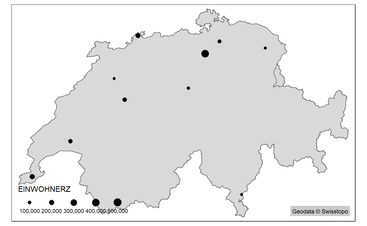

Now if you would want to include a swiss raster map into this plot you would:

first decide on a scale
look for the relevant map numbers based on the division (“Blatteinteilung”)
find the appropriate raster map files based on the map numbers from the previous step
import raster into R
check raster resolutions and possibly resample all rasters to same resolution
merge all the relevant raster maps into a single file
possibly reassign CRS and colormap

This package automates steps 2 - 7 with the function get_raster(). The function takes an sf object as an input. In addition, scale level (a scale 1:1’000’000 is defined as scale = 1000).

rastermap <- get_raster(features = switzerland,name = "relief")

## Using scale level:  1000

## Collective Size of Rasters to harmonize: 7.043344 (mb)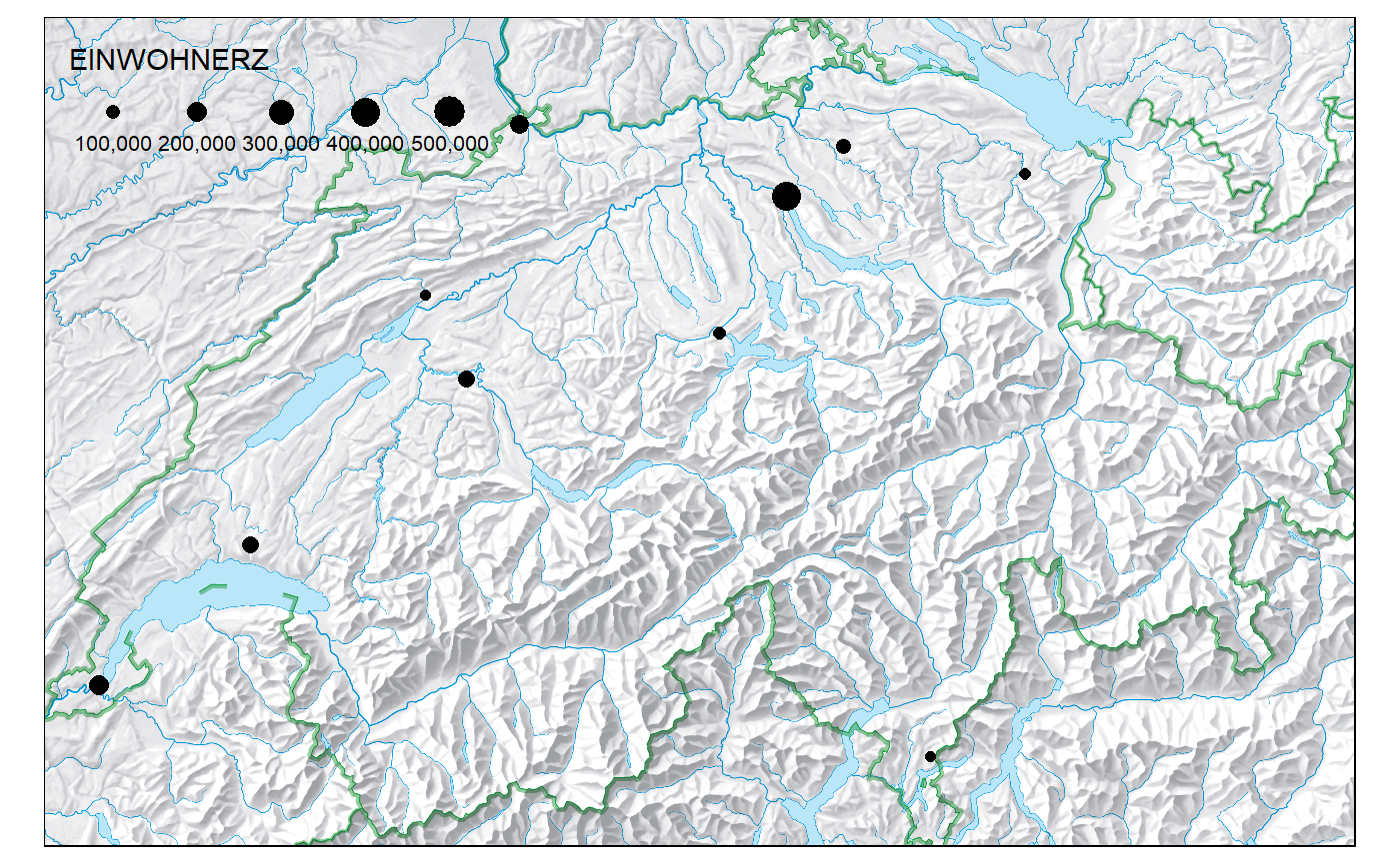

tm_shape(rastermap) + 
  tm_rgb() + 
  tm_shape(sample_points) + 
  tm_dots(size = "EINWOHNERZ")

Retrieve raster (example 2)

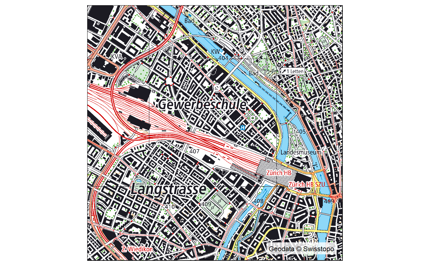
In the previous example, the function get_raster() basically called the whole raster file of the 1:100’000 raster map. The function is not particularly useful for such a use case. It becomes very useful however, when we want a custom extent possibly spanning over multiple rasters. This case is illustrated in the next example:

rastermap <- get_raster(sample_points[1,],x_add = 1000,y_add = 1000)

## Using scale level:  25

## Collective Size of Rasters to harmonize: 15.883634 (mb)

tm_shape(rastermap) + 
  tm_raster() + 
  tm_credits(credits("swisstopo"),bg.color = "white",bg.alpha = 0.8)